Demystifying “Matrix Capsules with EM Routing.”
Recently, Geoffrey Hinton, one of the fathers of deep learning, made waves in the machine learning community by publishing a revolutionary computer vision architecture: capsule networks. Hinton has been pushing for using capsule networks since 2012, after he first revolutionized the use of Convolutional Neural Networks (CNNs) for image detection, but only now has he made them feasible. The initial successful approach, published two weeks ago, is titled “Dynamic Routing Between Capsules.” Dynamic routing - which we’ll be exploring in depth throughout this post - allows networks to more intuitively understand part-whole relationships.
In the three days following the release of this paper, another paper on dynamic routing in capsule networks was submitted for review to ICLR 2018. This paper, titled “Matrix Capsules for EM Routing,” is widely speculated to have been authored by Hinton, and discusses a revolutionary new method for dynamic routing - even compared to his first paper. Although this approach shows significant promise, there’s been relatively less media attention surrounding it thus far. Because of the uncertainty of authorship, I refer to “the authors” for the rest of this post.
In this blog post, I’ll be discussing the intuition behind dynamic routing for matrix capsules and the mechanism for dynamic routing. The first part will outline the intuition for capsule networks and how they leverage dynamic routing to be more effective than traditional CNNs. The second part will take a deeper dive into the mathematical and technical details of EM Routing.
(Note: If you’ve read Sabour et. al., “Dynamic Routing Between Capsules,” the intuition is quite similar but the routing mechanism is very different.)
What’s Wrong with CNNs?
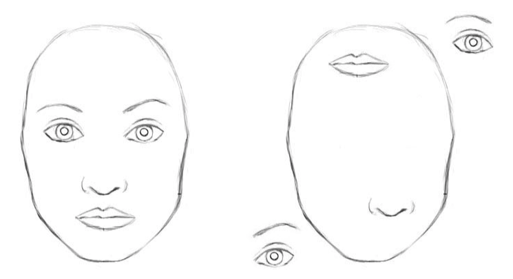
Since 2012, when Hinton co-authored a paper introducing AlexNet, a CNN that performed better than any previous method on image classification for ImageNet, CNNs have been the standard method for computer vision. In essence, CNNs work by detecting the presence of features in an image, and using the knowledge of these features to predict whether an object exists. However, CNNs only detect the existence of features - so even the image to the right, which contains a misplaced eye, nose, and ear, would be considered a face because it consists of all the necessary features!
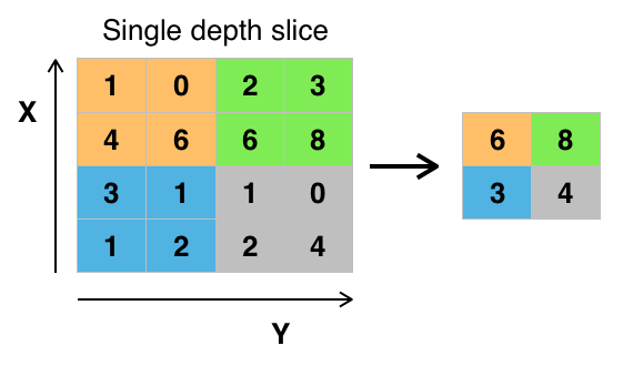
The reason for CNNs failure to deal with such images is the reason why Hinton has criticized CNNs for the last several years. The problem boils down to the way CNNs pass information from layer to layer: max pooling. Max pooling examines a grid of pixels, and takes the maximum activation in that region. This procedure essentially detects whether a feature is present in any region of the image, but loses spatial information about the feature.
Capsule networks attempt to address the limitations of CNNs by capturing part-whole relationships. For example, in a face, each of the two eyes is part of a forehead. In order to understand these part-whole relationships, capsule networks need to know more than just whether a feature exists - it needs to know where the feature is, how it is oriented, and other similar information. Capsule networks succeed in ways that CNNs have not because they successfully capture this information and route information from parts to their wholes.
So, What Exactly is a Capsule Network?
A traditional neural network is made up of neurons. Capsule networks impose structure on a CNN by grouping neurons into modules called capsules.
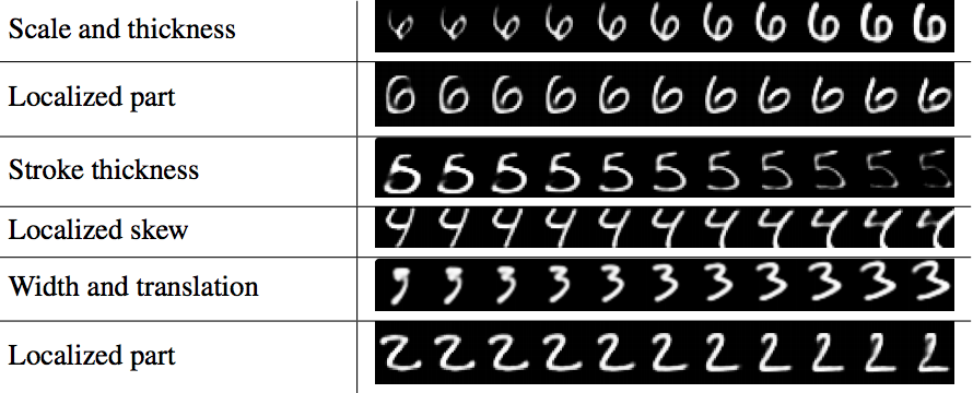
Capsules are groups of neurons whose output represents different properties of the same feature. By grouping neurons, the output of a capsule is a 4x4 matrix (or 16 dimensional vector), whose entries represent information such as the x and y-coordinates of the feature, the angle of rotation of the object, and other characteristics. For example, in digit recognition, one layer of capsules correspond to digits. One capsule in the output layer may correspond to a 6. Different entries in the 4x4 matrix will correspond to different properties of the 6. As seen below, if you modify one entry of the matrix, the 6 changes in scale and thickness, and if you modify another entry of the matrix, the top hook of the six changes.
When thinking of neural networks, we think in terms of connections between neurons. Although capsules are made up of neurons, it’s easier (and more effective) to think of the network as made up of components called capsules. The entire capsule network consists of layers of capsules. Each layer may consist of any number of capsules (often 8–32).
It is intuitively helpful to compare capsules to neurons in a traditional neural network. A single neuron in a NN outputs an activation from (0,1), and represents the existence of a feature. On the other hand, a capsule outputs a logistic unit (0,1) about the existence of a feature as well as a 4x4 matrix representing additional information about the feature. This 4x4 matrix is called the pose matrix because it represents spatial information about a feature. The diagram above illustrates what happens when you modify entries in the pose matrix.
In addition, we can consider neuron-neuron connections versus capsule-capsule connections, which would be represented by an single arrow in a typical diagram. In a NN, one neuron is connected to the next using a scalar weight. On the other hand, the connection between two capsules is now a 4x4 transformation matrix, because both the inputs and outputs of a capsule are 4x4 matrices!
So far, capsule networks haven’t done anything revolutionary: after all, capsules are often just convolutional layers. The effectiveness of capsule networks comes from the way information is transferred from layer to layer - what’s called a routing mechanism. Unlike CNNs, which route information using max pooling, capsule networks use a new process called dynamic routing to capture part-whole relationships.
Dynamic Routing Through Agreement: From Part to Whole
In this section, we’ll consider how to route outputs from layer (l) to layer (l+1). This procedure replaces max pooling from CNNs. Remember, as we discussed previously, our network learns transformation matrices (analogous to weights) as the connections between capsules. However, in addition to using these transformation matrices to route information from layer to layer, each connection is also multiplied by a routing coefficient that is dynamically computed. Don’t worry if this isn’t clear yet; we’ll first move through the intuition behind these routing coefficients, and then discuss the math later.
To make our analysis more concrete, we consider the example of digit recognition, and only classify the numbers 2 and 3. Our hidden layer (l) consists of a capsule layer with six capsules, corresponding to features, and our final layer (l+1) consists of 2 capsules, corresponding to the numbers 2 or 3. The features in layer (l) represent different components of the numbers 2 and 3. Suppose, for the sake of illustration, that our six capsule nodes to correspond to the following features. A 3 is composed of the first four features, and a 2 is composed of the first, fifth, and sixth features. In our example, our network will have taken an input image of 3, and will try to classify it.
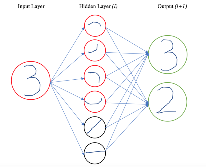
Intuitively, we know that every object in layer (l) comes from one of the higher-level objects in layer (l+1). We know that the first capsule is active in our network because it is either a 2 or a 3. Our goal is to figure out the probability that our feature is activated because of each feature in the next layer. Based on why we think capsules in layer (l) are being activated, we can direct our information from layer (l) to (l+1).
The question becomes how we decide these probabilities. Let’s take the example of the first capsule feature, which could be a part of a 2 or a 3. The number that it comes from depends largely on the spatial relationships between the first feature and other features in the layer. In our example, layer (l) sees the first feature (in the image) above the second feature above the third feature above the fourth. (Note: our pose matrix outputs can capture these spatial relationships between the features). So, layer (l) has seen all the information about a 3 with the correct relationships. If so, then there is significant agreement among layer (l) that a 3 is present. At the same time, the two other nodes for 2 are not active, so there is relatively less agreement that there is a two in the picture. Based on this agreement, we can say with high probability that the first feature actually came from a 3, not a 2.
This overall concept is called routing by agreement. By doing this, information from capsules in layer (l) is only supplied to layer (l+1) if the feature appears to have come from that capsule in the subsequent layer. In other words, the 2 capsule only receives information from the first feature if there’s more agreement about the 2. This procedure of dynamically computing which higher-level capsules to send information to is called dynamic routing. By dynamically routing the first feature (top hook) only to the 3, we can be more confident about our prediction and assign low probability to a 2.
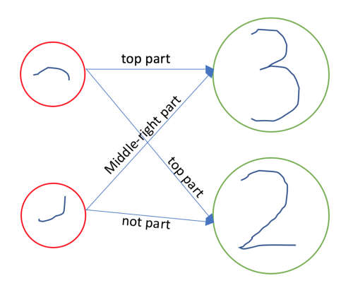
Here’s the trickiest part of dynamic routing: these routing coefficients are not learned parts of a network! The next three paragraphs will explain why. Our learned weights in capsule networks are the transformation matrices - analogous to weights in a NN. These transformation matrices can capture how each feature is related to the whole. For example, this can teach us that the first feature is the top of a 3 or the top of a 2, that the second feature is the middle-right of a 3, and so on.
However, we don’t know whether the first feature is part of a 3 or a 2, given the individual image. If there’s significant agreement that the different parts of a 3 relate properly to the whole, then we think the first feature should be routed to a 3. Other times, though, we might think its part of a two. As a result, it depends on the individual image whether the first feature is part of a 2 or a 3. These routing coefficients are consequently not fixed weights; they are learned every single forward pass of the network, and depend on the individual image. This is why the procedure is called dynamic routing - it is part of the forward pass.
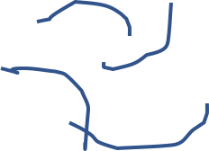
Let’s consider how this fixes the example when features aren’t in the right places, which had caused a problem for CNNs. The dynamic routing process is what helps fix this issue. Consider when the four features of a 3 are randomly placed in an input, as to the left. A convolutional network would consider this a 3, because it has the four components of a 3. However, in a capsule network, the “3 capsule” would receive information from the hidden layer saying that the parts of the 3 do not properly relate to form a 3! So, when the first capsule is deciding where to route its output, it does not see agreement for either the 2 or the 3, and sends its output equally. As a result, the capsule network does not predict either a 2 or a 3 with confidence. Hopefully, this shows why the routing must by dynamic, because it depends on the poses of the features activated by the capsule network.
As we showed above, this routing is only possible because the output of each capsule is a 4x4 matrix. These matrices capture the spatial relationships between the different parts of a 3, and if they do not agree correctly as parts of a whole, the capsule network does not route information with confidence. On the other hand, with CNNs, scalar activations cannot capture the relationship between each part and the whole.
Another way to frame dynamic routing is the concept of voting. Each capsule in layer (l) can vote which capsule in layer (l+1) it thinks it came from. The capsule gets a total of one vote, and can distribute this vote fractionally among all subsequent layer capsules. This voting mechanism ensures effective routing of information based on spatial relationships. The voting/routing mechanism comes from the procedure that is discussed below.
EM Routing: Overall Idea
We’ve vaguely outlined the intuition behind dynamic routing, but have said nothing about how to compute it. This topic is lengthy and complex, and will be covered in full mathematical detail in the next part of this series. Here, I’ll outline the basic idea behind EM Routing.
Essentially, when routing, we are making the assumption that each capsule in layer (l) is activated because it is part of some ‘whole’ in the next layer. In this step, we assume there is some latent variable that explains which ‘whole’ our information came from, and are trying to infer the probability that each matrix output came from the higher-order feature in level (l+1).
This boils down to an unsupervised learning problem, and we tackle it with an algorithm called Expectation Maximization. In essence, expectation maximization attempts to maximize the likelihood that our data (outputs of layer (l)) is explained by the capsules in layer (l+1). Expectation Maximization is an iterative algorithm that consists of two steps: expectation, and maximization. Typically, for capsule networks, each step is performed three times, and then terminated.
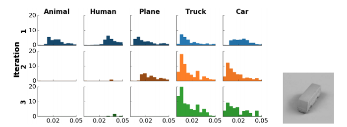
The authors explain the steps are as follows. Expectation assigns probabilities that each capsule in layer (l) was explained by the capsules in layer (l+1). Then, the maximization step decides whether the capsules in layer (l+1) are active, if they see significant clustering of inputs to it (agreement), and decides what the input is to the capsule by taking a weighted average of the routed inputs.
Don’t worry if this didn’t make sense - I explained a lot of dense math in very few words. If you want to understand the deep technicalities of the routing mechanism, stay tuned for the next blog post later this week.
Capsule Network Architecture
Now that we understand the intuition behind capsule networks, we can examine how the authors used matrix capsules in their paper “Matrix Capsules with EM Routing.”
The paper evaluates matrix capsules on the SmallNORB dataset. This dataset consists of five types of children’s toys photographed from different angles and elevations. The dataset accurately captures different viewpoints of the same object. Recall that capsules are fundamentally better at understanding viewpoints because of the multidimensional output of capsules (pose matrices)- this is why the SmallNORB dataset is an excellent evaluation metric for the goals of Capsule Networks.
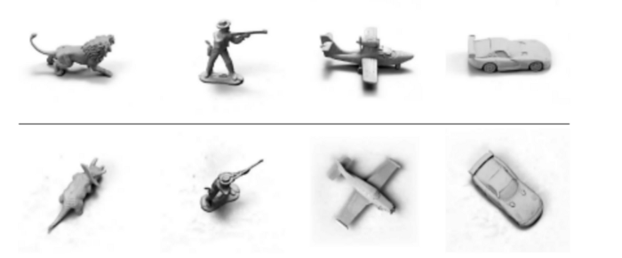
The architecture consists of a convolutional layer, followed by two capsule layers, and a final classification capsule layer with five capsules, one per class. This architecture performs better than any previous model on the dataset and cuts the previous best error rate by over 45%!

Advantages of Capsule Networks
Capsule networks have four major conceptual advantages over CNNs.
- Viewpoint Invariance. As discussed throughout this piece, the use of pose matrices allows capsule networks to recognize objects regardless of the viewpoint from which they are viewed.
- Fewer Parameters. Because matrix capsules group neurons, the connections between layers require fewer parameters. The model that achieved the best performance only included 300,000 parameters, as compared with the 4,000,000 parameters of their baseline CNN. This means the model can generalize better.
- Better generalization to new viewpoints. CNNs, when trained to understand rotations, often memorize that an object can be viewed similarly from several different rotations. However, capsule networks also generalize better to new viewpoints because pose matrices can capture these characteristics as mere linear transformations.
- Defense against white-box adversarial attacks. The Fast Gradient Sign Method (FGSM) is a typical method for attacking CNNs. It evaluates the gradient of each pixel against the loss of the network, and changes each pixel by at most epsilon to maximize the loss. Although this method can drop the accuracy of CNNs dramatically, to below 20%, capsule networks maintain an accuracy of above 70%.
In this post, I discuss some details specific to matrix capsules. The details of using matrix capsules with EM routing, instead of using vector capsules in the initial paper, also present three major benefits. I explain the technical details of these three benefits in my next post.
The Future of Computer Vision
It’s been two weeks since capsule networks have been introduced, and nobody knows whether they’re another model that people will forget, or if they will revolutionize computer vision. In their current state, they have plenty of drawbacks - most notably the extensive time required to dynamically route using EM from layer to layer. This can be especially problematic when parallelizing over GPUs.
Regardless, this paper effectively acted as a proof of concept for capsule networks, and did so quite elegantly. In the future, though, their efficacy must be tested on a wide variety of datasets, including more applicable ones with many classes, such as ImageNet. Over time, new routing mechanisms may be introduced, and other innovations may make capsule nets more efficient (we’ve already seen this in “Matrix Capsules with EM Routing,” which completely changed the routing mechanism!). If they work, though, the applications are endless - to image classification, object detection, dense captioning, generative networks, and few-shot learning.
Acknowledgements — A huge thanks to Shubhang Desai, Adi Ganesh, Jeffrey Chang, and Jordan Alexander for giving me excellent feedback on this post. Check out the original papers here and here.
This post is migrated from the original Medium post, which you can see here.

Comments